Jupyter Notebook example
Creating a cube
This example will create a 500x500 pixels cube with the 12-bands images from S-PLUS TILE HYDRA-0045 for the NGC3312 galaxy. The stamps are made from a cropped 500x500 pixels area located at S-PLUS TILE mentioned before, centered at coordinates RA 10h37m02.5s and DEC -27d33’56”.
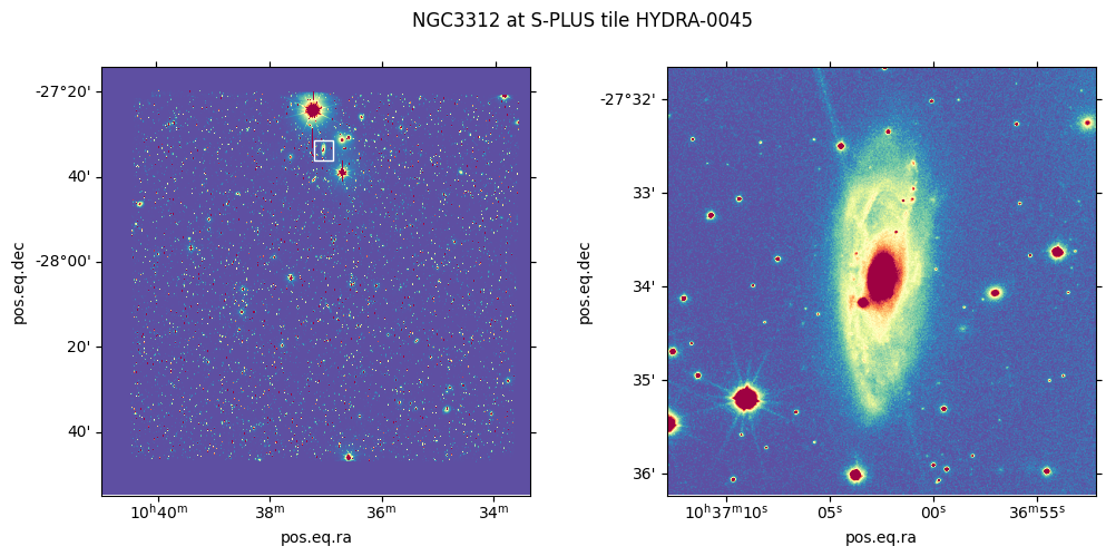
NGC3312 crop at HYDRA-0045 S-PLUS tile
The scubes entry-point script will download the 12-band stamps and
calculate the fluxes and errors of each image. The images are zero-point
calibrated based on the S-PLUS iDR4 (scubes package includes zp
data) values, but they are not corrected for Galactic extinction.
The resultant files will be created at directory workdir.
The program also could use SExtractor in order to create a spatial mask of stars, attempting to remove the areas enclosed by the brightest ones along the FOV (-M optional argument). To use this option, do not forget to include the SExtractor executable path using the option -x. An example of this usage could be find at: Mask stars with scubes package.
scubes entry-point script help and usage:
!scubes --help
usage: scubes [-h] [-r] [-c] [-f] [-b BANDS [BANDS ...]] [-l SIZE] [-N]
              [-w WORK_DIR] [-o OUTPUT_DIR] [-x SEXTRACTOR] [-p CLASS_STAR]
              [-v] [-D] [-S SATUR_LEVEL] [-Z ZPCORR_DIR] [-z ZP_TABLE]
              [-B BACK_SIZE] [-T DETECT_THRESH] [-U USERNAME] [-P PASSWORD]
              [-M] [-I] [-F] [-R] [--version]
              SPLUS_TILE RA DEC GALAXY_NAME

┌─┐   ┌─┐┬ ┬┌┐ ┌─┐┌─┐  | Create S-PLUS galaxies data cubes, a.k.a. S-CUBES.
└─┐───│  │ │├┴┐├┤ └─┐  | S-CUBES is an organized FITS file with data, errors,
└─┘   └─┘└─┘└─┘└─┘└─┘  | mask and metadata about some galaxy present on any
---------------------- + S-PLUS observed tile. Any problem contact:

   Eduardo Alberto Duarte Lacerda <dhubax@gmail.com>, Fabio Herpich <fabiorafaelh@gmail.com>

The input values of RA and DEC will be converted to degrees using the
scubes.utilities.io.convert_coord_to_degrees(). All scripts with RA
and DEC inputs parse angles in two different units:

- hourangle: using hms divisors; Ex: 10h37m2.5s
- degrees: using : or dms  divisors; Ex: 10:37:2.5 or 10d37m2.5s

Note that 10h37m2.5s is a totally different angle from 10:37:2.5
(159.26 deg and 10.62 deg respectively).

positional arguments:
  SPLUS_TILE                  Name of the S-PLUS tile
  RA                          Galaxy's right ascension
  DEC                         Galaxy's declination
  GALAXY_NAME                 Galaxy's name

options:
  -h, --help                  show this help message and exit
  -r, --redo                  Enable redo mode to overwrite final cubes.
                              Default value is False
  -c, --clean                 Clean intermediate files after processing.
                              Default value is False
  -f, --force                 Force overwrite of existing files. Default value
                              is False
  -b BANDS [BANDS ...], --bands BANDS [BANDS ...]
                              List of S-PLUS bands (space separated). Default
                              value is ['U', 'F378', 'F395', 'F410', 'F430',
                              'G', 'F515', 'R', 'F660', 'I', 'F861', 'Z']
  -l SIZE, --size SIZE        Size of the cube in pixels. If size is a odd
                              number, the program will choose the closest even
                              integer. Default value is 500
  -N, --no_interact           Run only the automatic stars mask (a.k.a. do not
                              check final mask) Default value is False
  -w WORK_DIR, --work_dir WORK_DIR
                              Working directory. Default value is /storage/hdd
                              /backup/dhubax/dev/astro/splus/s-cubes/workdir
  -o OUTPUT_DIR, --output_dir OUTPUT_DIR
                              Output directory. Default value is /storage/hdd/
                              backup/dhubax/dev/astro/splus/s-cubes/workdir
  -x SEXTRACTOR, --sextractor SEXTRACTOR
                              Path to SExtractor executable. Default value is
                              sex
  -p CLASS_STAR, --class_star CLASS_STAR
                              SExtractor CLASS_STAR parameter for star/galaxy
                              separation. Default value is 0.25
  -v, --verbose               Verbosity level.
  -D, --debug                 Enable debug mode. Default value is False
  -S SATUR_LEVEL, --satur_level SATUR_LEVEL
                              Saturation level for the png images. Default
                              value is 1600.0
  -Z ZPCORR_DIR, --zpcorr_dir ZPCORR_DIR
                              Zero-point correction directory. Default value
                              is /home/lacerda/.local/lib/python3.10/site-
                              packages/scubes/data/zpcorr_iDR4
  -z ZP_TABLE, --zp_table ZP_TABLE
                              Zero-point table. Default value is
                              /home/lacerda/.local/lib/python3.10/site-
                              packages/scubes/data/iDR4_zero-points.csv
  -B BACK_SIZE, --back_size BACK_SIZE
                              Background mesh size for SExtractor. Default
                              value is 64
  -T DETECT_THRESH, --detect_thresh DETECT_THRESH
                              Detection threshold for SExtractor. Default
                              value is 1.1
  -U USERNAME, --username USERNAME
                              S-PLUS Cloud username.
  -P PASSWORD, --password PASSWORD
                              S-PLUS Cloud password.
  -M, --mask_stars            Run SExtractor to auto-identify stars on stamp.
                              Default value is False
  -I, --det_img               Downloads detection image for the stamp. Needed
                              if --mask_stars is active. Default value is
                              False
  -F, --estimate_fwhm         Runs SExtractor two times estimating the
                              SEEING_FWHM of the detection image. Default
                              value is False
  -R, --remove_downloaded_data
                              Remove the downloaded data from splusdata at the
                              end of the run. Default value is False
  --version                   show program's version number and exit
The call to the entry-point script scubes to this example would be:
Do not forget to change YOURUSER and YOURPASS for your credentials at S-PLUS Cloud.
!scubes -fR -w . -U YOURUSER -P YOURPASS -l 500 -- HYDRA-0045 10h37m02.5s -27d33\'56\" NGC3312
NGC3312 @ HYDRA-0045 - downloading: 100%|███████| 12/12 [00:29<00:00,  2.42s/it]
WARNING: FITSFixedWarning: 'datfix' made the change 'Set DATE-OBS to '2017-02-19' from MJD-OBS'. [astropy.wcs.wcs]
[2024-05-26T19:17:59.990086] - scubes: Reading ZPs table: /home/lacerda/.local/lib/python3.10/site-packages/scubes/data/iDR4_zero-points.csv
[2024-05-26T19:17:59.993503] - scubes: Getting ZP corrections for the S-PLUS bands...
[2024-05-26T19:17:59.998823] - scubes: Calibrating stamps...
/home/lacerda/.local/lib/python3.10/site-packages/scubes/core.py:523: RuntimeWarning: cdelt will be ignored since cd is present
  nw.wcs.cdelt[:2] = w.wcs.cdelt
[2024-05-26T19:18:00.781773] - scubes: Cube successfully created!
[2024-05-26T19:18:00.781793] - scubes: Removing downloaded data
How to read a cube
A cube resultant from scubes script is stored using FITS format and
is called SCUBE. In order to help the user, scubes package
implements a utility class to read the SCUBE. This class implements
the method lRGB_image() to create Lupton RGB images.
Below an example of the scubes.utilities.read_scube() usage:
from os.path import join
from scubes.utilities.readscube import read_scube

SNAME = f'NGC3312'
filename = join(SNAME, f'{SNAME}_cube.fits')

scube = read_scube(filename)
Headers
The PRIMARY HEADER (scube.primary_header) contains information
about the object, all processed by the code. The DATA HEADER
(scube.data_header) otherwise, includes information about the tile
observation and a 3D World Coordinate System (WCS) information, which is
converted to a 2D astropy.wcs.WCS() instance in the variable
scube.wcs.
scube.primary_header
SIMPLE  =                    T / conforms to FITS standard
BITPIX  =                    8 / array data type
NAXIS   =                    0 / number of array dimensions
EXTEND  =                    T
TILE    = 'HYDRA-0045'
GALAXY  = 'NGC3312 '
SIZE    =                  500 / Side of the stamp in pixels
X0TILE  =             5683.973
Y0TILE  =             8849.952
RA      =   159.26041666666666
DEC     =  -27.565555555555555
scube.data_header
XTENSION= 'IMAGE   '           / Image extension
BITPIX  =                  -64 / array data type
NAXIS   =                    3 / number of array dimensions
NAXIS1  =                  500
NAXIS2  =                  500
NAXIS3  =                   12
PCOUNT  =                    0 / number of parameters
GCOUNT  =                    1 / number of groups
COMMENT   FITS (Flexible Image Transport System) format is defined in 'Astronomy
COMMENT   and Astrophysics', volume 376, page 359; bibcode: 2001A&A...376..359H
EQUINOX =        2000.00000000 / Mean equinox
MJD-OBS =   5.780300000000E+04 / [d] MJD of observation
RADESYS = 'ICRS    '           / Equatorial coordinate system
CTYPE1  = 'RA---TAN'           / Coordinate type code
CUNIT1  = 'deg     '           / Units of coordinate increment and value
CRVAL1  =   1.592920354170E+02 / Coordinate value at reference point
CRPIX1  = 6.850000000000000E+01 / Pixel coordinate of reference point
CD1_1   =  -1.527777777778E-04 / Linear projection matrix
CD1_2   =   0.000000000000E+00 / Linear projection matrix
CTYPE2  = 'DEC--TAN'           / Coordinate type code
CUNIT2  = 'deg     '           / Units of coordinate increment and value
CRVAL2  =  -2.807726741670E+01 / Coordinate value at reference point
CRPIX2  = -3.097500000000000E+03 / Pixel coordinate of reference point
CD2_1   =   0.000000000000E+00 / Linear projection matrix
CD2_2   =   1.527777777778E-04 / Linear projection matrix
EXPTIME =                  1.0 / Normalized exposure time
SATURATE=   2.830922105506E+02 / Saturation Level (ADU)
COMMENT
SOFTNAME= 'SWarp   '           / The software that processed those data
SOFTVERS= '2.38.0  '           / Version of the software
SOFTDATE= '2017-01-17'         / Release date of the software
SOFTAUTH= '2010-2012 IAP/CNRS/UPMC' / Maintainer of the software
SOFTINST= 'IAP  http://www.iap.fr' / Institute
COMMENT
AUTHOR  = 'jype    '           / Who ran the software
ORIGIN  = 't80s-jype4'         / Where it was done
DATE    = '2019-01-31T17:38:35' / When it was started (GMT)
COMBINET= 'WEIGHTED'           / COMBINE_TYPE config parameter for SWarp
COMMENT
COMMENT  Propagated FITS keywords
OBJECT  = 'NGC3312 '           / name of observed object
TELESCOP= 'T80     '           / Telescope Model
INSTRUME= 'T80Cam  '           / Custom. Name of instrument
COMMENT
COMMENT  Axis-dependent config parameters
RESAMPT1= 'LANCZOS3'           / RESAMPLING_TYPE config parameter
CENTERT1= 'MANUAL  '           / CENTER_TYPE config parameter
PSCALET1= 'MANUAL  '           / PIXELSCALE_TYPE config parameter
RESAMPT2= 'LANCZOS3'           / RESAMPLING_TYPE config parameter
CENTERT2= 'MANUAL  '           / CENTER_TYPE config parameter
PSCALET2= 'MANUAL  '           / PIXELSCALE_TYPE config parameter
        STATS 2019-01-31T14:40:30.666269
HIERARCH OAJ QC NCMODE = 0.0 / Mode (ADU)
HIERARCH OAJ QC NCMIDPT = 0.0001 / Level estim (ADU)
HIERARCH OAJ QC NCMIDRMS = 0.000599999999999999 / rms level (ADU)
HIERARCH OAJ QC NCNOISE = 0.0073 / Noise estim (ADU)
HIERARCH OAJ QC NCNOIRMS = 0.0005 / rms noise estim (ADU)
        FWHM ESTIM 2019-01-31T14:41:27.247078
HIERARCH OAJ PRO FWHMSEXT = 1.578 / FWHM arcsec estimated with SE
HIERARCH OAJ PRO FWHMSRMS = 0.07199999999999999 / rms in FWHM with SE
HIERARCH OAJ PRO FWHMBETA = 2.332319974899292 / PSFex beta
HIERARCH OAJ PRO FWHMNSTARS = 405 / PSFex nstars
HIERARCH OAJ PRO ELLIPMEAN = 0.02642080001533031 / PSFex Ellip
PIXSCALE=                 0.55
FILENAME= 'HYDRA-0045_U_swp.fits'
TEXPOSED=               1362.0
TEXPSUM =               1362.0 / Maximum equivalent exposure time (s)
HIERARCH OAJ PRO PIPVERS = '0.9.9   '
HIERARCH OAJ PRO REFIMAGE = 'HYDRA_C-20170328-044356_proc' / Reference image for
HIERARCH OAJ PRO REFAIRMASS = 1.080421306670953 / Reference image airmass
HIERARCH OAJ PRO REFDATEOBS = '2017-03-28T04:39:52.019000' / Reference image dat
HIERARCH OAJ PRO SWCMB1 = 'HYDRA_C-20170219-055302_proc'
HIERARCH OAJ PRO SWSCALE1 = 0.004404859185018
HIERARCH OAJ PRO SWCMB2 = 'HYDRA_C-20170219-055728_proc'
HIERARCH OAJ PRO SWSCALE2 = 0.004405737992425
HIERARCH OAJ PRO SWCMB3 = 'HYDRA_C-20170219-060145_proc'
HIERARCH OAJ PRO SWSCALE3 = 0.004423817580924
HIERARCH OAJ PRO SWCMB4 = 'HYDRA_C-20170328-043935_proc'
HIERARCH OAJ PRO SWSCALE4 = 0.00405233218495
HIERARCH OAJ PRO SWCMB5 = 'HYDRA_C-20170328-044356_proc'
HIERARCH OAJ PRO SWSCALE5 = 0.00404267877143
HIERARCH OAJ PRO SWCMB6 = 'HYDRA_C-20170328-044814_proc'
HIERARCH OAJ PRO SWSCALE6 = 0.00407020637223
HISTORY Image was compressed by CFITSIO using scaled integer quantization:
HISTORY   q = 4.000000 / quantized level scaling parameter
HISTORY 'SUBTRACTIVE_DITHER_1' / Pixel Quantization Algorithm
CHECKSUM= 'bC4fbC4fbC4fbC4f'   / HDU checksum updated 2019-01-31T17:52:34
DATASUM = '1624960924'         / data unit checksum updated 2019-01-31T17:52:34
X01TILE =                249.5 / Center position
Y01TILE =                249.5 / Center position
X0TILE  =             5683.973 / Center position
Y0TILE  =             8849.952 / Center position
TILE    = 'HYDRA-0045'
WCSAXES =                    3 / Number of coordinate axes
PC1_1   =  -0.0001527777777778 / Coordinate transformation matrix element
PC2_2   =   0.0001527777777778 / Coordinate transformation matrix element
CDELT1  =                 1.0  / Coordinate increment at reference point
CDELT2  =                 1.0  / Coordinate increment at reference point
LONPOLE =                180.0 / [deg] Native longitude of celestial pole
LATPOLE =                 90.0 / [deg] Native latitude of celestial pole
MJDREF  =                  0.0 / [d] MJD of fiducial time
DATE-OBS= '2017-02-19'         / ISO-8601 time of observation
CRPIX3  =                  0.0 / Pixel coordinate of reference point
CDELT3  =                  1.0 / Coordinate increment at reference point
CRVAL3  =                  0.0 / Coordinate value at reference point
EXTNAME = 'DATA    '           / Name of the extension
BUNIT   = 'erg / (Angstrom s cm2)' / Physical units of the array values
2D WCS instance:
scube.wcs
/home/lacerda/.local/lib/python3.10/site-packages/astropy/wcs/wcs.py:3137: RuntimeWarning: cdelt will be ignored since cd is present
  description.append(s.format(*self.wcs.cdelt))
WCS Keywords

Number of WCS axes: 2
CTYPE : 'RA---TAN'  'DEC--TAN'
CRVAL : 159.292035417  -28.0772674167
CRPIX : 68.5  -3097.5
PC1_1 PC1_2  : -0.0001527777777778  0.0
PC2_1 PC2_2  : 0.0  0.0001527777777778
CDELT : 1.0  1.0
NAXIS : 500  500  12
Filters information
scubes includes some information about the filters used to obtain
S-PLUS images. The script is called scubes_filters and the data is
obtained from S-PLUS Filters Transmission Curve
Calculator, made
by Fabio Herpich.
!scubes_filters --decimals 2
filter central_wave delta_wave trapz_wave trapz_width mean_wave mean_width mean_1_wave mean_1_width pivot_wave alambda_av
------ ------------ ---------- ---------- ----------- --------- ---------- ----------- ------------ ---------- ----------
 uJAVA      3576.59     324.89    3542.14      322.83   3542.14     322.83     3541.97       322.48    3533.28       1.61
 J0378      3770.67     150.99    3774.01      135.96   3774.01     135.96     3773.98       135.75    3773.16       1.52
 J0395      3940.67      102.8    3941.09      100.78   3941.09     100.78     3941.07       100.66     3940.7       1.46
 J0410      4094.08     200.31    4096.24      193.35   4096.24     193.35     4096.21       193.12    4094.93        1.4
 J0430      4292.02     200.16    4293.38      195.07   4293.38     195.07     4293.34       194.82    4292.11       1.33
 gSDSS      4774.03    1505.46     4821.1     1312.44    4821.1    1312.44     4821.07      1312.17    4758.49        1.2
 J0515      5132.82     207.06    5134.22      203.61   5134.22     203.61      5134.2       203.48    5133.13        1.1
 rSDSS      6274.74    1436.69    6295.69     1274.09   6295.69    1274.09     6295.67      1273.72    6251.83       0.86
 J0660      6613.99     147.28    6614.32      146.67   6614.32     146.67      6614.3       146.52    6613.88        0.8
 iSDSS       7702.5    1506.85    7709.96      1438.1   7709.96     1438.1     7709.81      1437.21    7670.61       0.65
 J0861      8611.48     409.69    8609.86      401.91   8609.87     401.91     8609.84       401.53    8607.25       0.54
 zSDSS       8881.7     1270.5    8985.81     1308.49   8985.81    1308.49     8986.54       1307.7    8941.48       0.51
The class scube also makes available some information about the
filters, such as:
scube.filters: filters names
scube.pivot_wave: pivot wavelenghts
scube.central_wave: central wavelenghts
for _f, _p, _c in zip(scube.filters, scube.pivot_wave, scube.central_wave):
    print(f'filter: {_f} wave(pivot, central): ({_p:.2f}, {_c:.2f})')
filter: uJAVA wave(pivot, central): (3533.28, 3576.59)
filter: J0378 wave(pivot, central): (3773.16, 3770.67)
filter: J0395 wave(pivot, central): (3940.70, 3940.67)
filter: J0410 wave(pivot, central): (4094.93, 4094.08)
filter: J0430 wave(pivot, central): (4292.11, 4292.02)
filter: gSDSS wave(pivot, central): (4758.49, 4774.03)
filter: J0515 wave(pivot, central): (5133.13, 5132.82)
filter: rSDSS wave(pivot, central): (6251.83, 6274.74)
filter: J0660 wave(pivot, central): (6613.88, 6613.99)
filter: iSDSS wave(pivot, central): (7670.61, 7702.50)
filter: J0861 wave(pivot, central): (8607.25, 8611.48)
filter: zSDSS wave(pivot, central): (8941.48, 8881.70)
More metadata about the SCUBE cube, such as the exposure times,
gains, PSF FWHM and the date of the observation can be found with
scube.metadata:
scube.metadata
FITS_rec([('uJAVA', 3576.5900319 , 3533.28150603, 1302.99580147, 2651.74575679, 1.4238565 , '2017-02-19'),
          ('J0378', 3770.66765668, 3773.16495619, 1266.43687077, 2590.53003934, 1.24601953, '2017-02-19'),
          ('J0395', 3940.66900669, 3940.69812172,  680.64843148, 1401.35102734, 1.18031096, '2017-02-19'),
          ('J0410', 4094.0795908 , 4094.92800733,  345.42806559,  706.83367717, 1.13351701, '2017-02-19'),
          ('J0430', 4292.0201202 , 4292.10579006,  278.90845694,  570.57617371, 1.14671147, '2017-02-19'),
          ('gSDSS', 4774.02604026, 4758.4878587 ,  191.4341835 ,  370.91141421, 1.2285185 , '2017-02-19'),
          ('J0515', 5132.82097321, 5133.13247975,  299.46581613,  610.78047227, 1.10798045, '2017-02-19'),
          ('rSDSS', 6274.74334743, 6251.83097429,  195.74024342,  396.72506048, 1.09843247, '2017-02-19'),
          ('J0660', 6613.99318993, 6613.87556039, 1430.33833785, 2904.99319306, 1.07404553, '2017-02-19'),
          ('iSDSS', 7702.49932499, 7670.61445983,  272.39806574,  560.98501139, 1.03689299, '2017-02-19'),
          ('J0861', 8611.48166482, 8607.25421702,  479.32598833,  984.36649508, 1.083632  , '2017-02-19'),
          ('zSDSS', 8881.70071701, 8941.47606623,  275.62079939,  566.9703096 , 1.03092001, '2017-02-19')],
         dtype=(numpy.record, [('FILTER', 'S5'), ('CENTWAVE', '>f8'), ('PIVOTWAVE', '>f8'), ('EXPTIME', '>f8'), ('GAIN', '>f8'), ('PSFFWHM', '>f8'), ('DATE-OBS', 'S10')]))
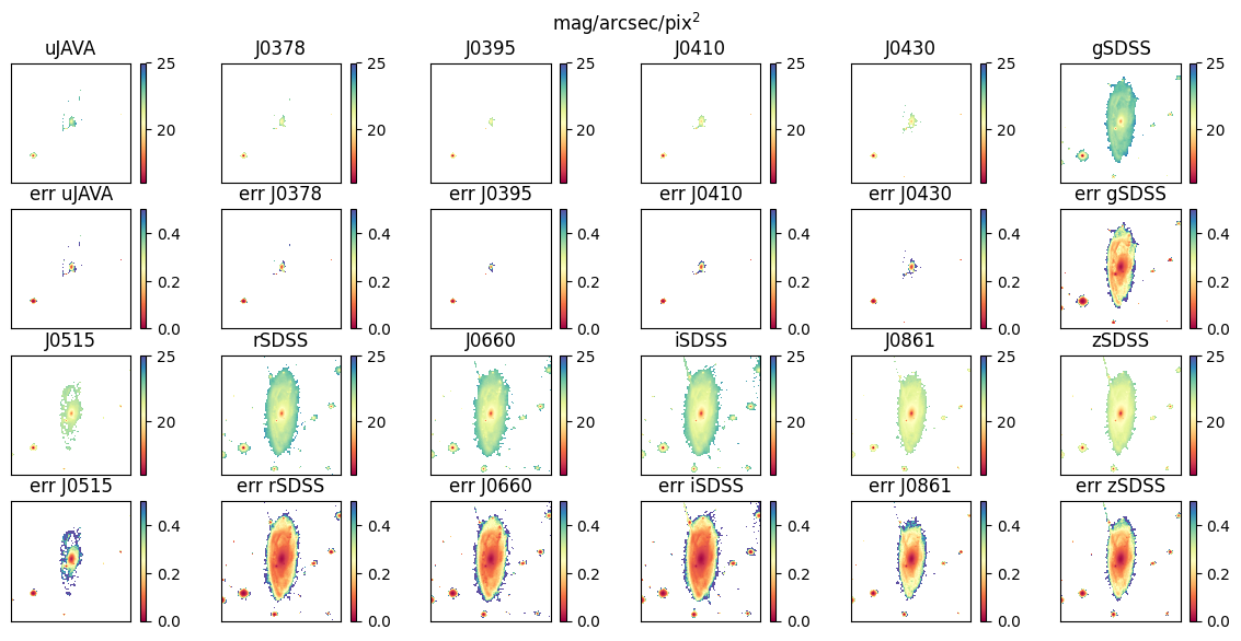
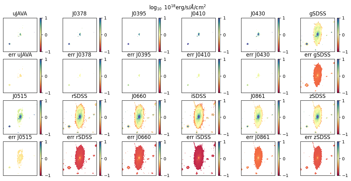
Images plot
This example below plots the images of the magnitudes and errors from
all filters, calculated by scubes package. The of the flux and
errors by default are in erg/s/\(\unicode{x212B}\)/cm\(^2\):
scube.flux__lyx and scube.eflux__lyx
the lyx suffix points the dimensions of the array (Lambda, Y, X).
scube class also create arrays with the value converted to
mag/arcsec/pix\(^2\):
scube.mag__lyx and scube.emag__lyx
import numpy as np
import matplotlib.pyplot as plt
import matplotlib.ticker as ticker
f__byx = scube.mag__lyx
ef__byx = scube.emag__lyx
weimask__yx = scube.weimask__yx
filters_names = scube.metadata['FILTER']
nb, ny, nx = f__byx.shape
nrows = 2
ncols = int(nb/nrows)
f, ax_arr = plt.subplots(2*nrows, ncols)
f.set_size_inches(12, 6)
f.subplots_adjust(left=0.01, right=0.95, bottom=0.05, top=0.90, hspace=0.22, wspace=0.13)
k = 0
for ir in range(nrows):
    for ic in range(ncols):
        img = f__byx[k]
        vmin, vmax = 16, 25
        ax = ax_arr[ir*2, ic]
        ax.set_title(filters_names[k])
        im = ax.imshow(img, origin='lower', cmap='Spectral', vmin=vmin, vmax=vmax)
        plt.colorbar(im, ax=ax)
        ax.xaxis.set_major_locator(ticker.NullLocator())
        ax.yaxis.set_major_locator(ticker.NullLocator())

        eimg = ef__byx[k]
        vmin, vmax = 0, 0.5
        ax = ax_arr[ir*2 + 1, ic]
        ax.set_title(f'err {filters_names[k]}')
        im = ax.imshow(eimg, origin='lower', cmap='Spectral', vmin=vmin, vmax=vmax)
        plt.colorbar(im, ax=ax)
        ax.xaxis.set_major_locator(ticker.NullLocator())
        ax.yaxis.set_major_locator(ticker.NullLocator())

        k += 1
f.suptitle(r'mag/arcsec/pix$^2$')
Text(0.5, 0.98, 'mag/arcsec/pix$^2$')
f__byx = np.ma.log10(scube.flux__lyx) + 18
ef__byx = np.ma.log10(scube.eflux__lyx) + 18
weimask__yx = scube.weimask__yx
filters_names = scube.metadata['FILTER']
nb, ny, nx = f__byx.shape
nrows = 2
ncols = int(nb/nrows)
f, ax_arr = plt.subplots(2*nrows, ncols)
f.set_size_inches(12, 6)
f.subplots_adjust(left=0.01, right=0.95, bottom=0.05, top=0.90, hspace=0.22, wspace=0.13)
k = 0
for ir in range(nrows):
    for ic in range(ncols):
        img = f__byx[k]
        vmin, vmax = np.percentile(img.compressed(), [5, 95])
        vmin, vmax = -1, 1
        ax = ax_arr[ir*2, ic]
        ax.set_title(filters_names[k])
        im = ax.imshow(img, origin='lower', cmap='Spectral', vmin=vmin, vmax=vmax)
        plt.colorbar(im, ax=ax)
        ax.xaxis.set_major_locator(ticker.NullLocator())
        ax.yaxis.set_major_locator(ticker.NullLocator())
        eimg = ef__byx[k]
        vmin, vmax = np.percentile(eimg.compressed(), [5, 95])
        vmin, vmax = -1, 1
        ax = ax_arr[ir*2 + 1, ic]
        ax.set_title(f'err {filters_names[k]}')
        im = ax.imshow(eimg, origin='lower', cmap='Spectral', vmin=vmin, vmax=vmax)
        plt.colorbar(im, ax=ax)
        ax.xaxis.set_major_locator(ticker.NullLocator())
        ax.yaxis.set_major_locator(ticker.NullLocator())

        k += 1
f.suptitle(r'$\log_{10}$ 10$^{18}$erg/s/$\AA$/cm$^2$')
Text(0.5, 0.98, '$\log_{10}$ 10$^{18}$erg/s/$\AA$/cm$^2$')
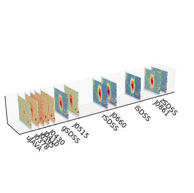
3D image
import astropy.units as u

xx, yy = np.meshgrid(range(scube.size), range(scube.size))
FOV = 140*u.deg
focal_lenght = 1/np.tan(FOV/2)
print(f'FOV: {FOV}\nfocal lenght: {focal_lenght}')
f = plt.figure()
ax = f.add_subplot(projection='3d')
for i, _w in enumerate(scube.pivot_wave):
    sc = ax.scatter(xx, yy, c=np.ma.log10(scube.flux__lyx[i]) + 18,
                    zs=_w, s=1, edgecolor='none', vmin=-1, vmax=0.5, cmap='Spectral_r')
ax.set_zticks(scube.pivot_wave)
ax.set_zticklabels(scube.filters, rotation=-45)
ax.set_proj_type('persp', focal_length=focal_lenght)
ax.set_box_aspect(aspect=(7, 1, 1))
ax.view_init(elev=20, azim=-125, vertical_axis='y')
ax.set_xticks([])
ax.set_yticks([])
for spine in ax.spines.values():
    spine.set_visible(False)
FOV: 140.0 deg
focal lenght: 0.36397023426620245
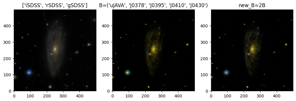
RGB and Filters plot
This series of examples below are using the Lupton RGB method of the
scube module and some of the data stored by the scubes
package in order to create a filters transmittance plot.
scubes package implements various constants in scubes.constants
module. This example below uses FILTER_NAMES_FITS,
FILTERS_COLORS and FILTER_TRANSMITTANCE data. The filters
transmittance curves are calculated by splus-filters package:
The scubes.utilities.read_scube.lRGB_image is a wrapper to
astropy.visualization.make_lupton_rgb() that creates RGB images
using the SCUBE instantiated by scubes.utilities.read_scube
class.
# RGB plot
rgb_f = [1, 1, 1]
pminmax = [5, 95]
Q = 10
stretch = 5
im_max = 1
minimum = (0, 0, 0)

f, axArr = plt.subplots(1, 3)
ax1, ax2, ax3 = axArr
f.set_size_inches(12, 4)

###### original RGB from splus.data package
rgb = ['iSDSS', 'rSDSS', 'gSDSS']
rgb__yxb = scube.lRGB_image(rgb, rgb_f, pminmax, Q=Q, stretch=stretch, im_max=im_max, minimum=minimum)
ax1.imshow(rgb__yxb, origin='lower')
ax1.set_title(rgb)

###### improved RGB
R_filters = 'iSDSS'
G_filters = 'rSDSS'
B_filters = tuple(scube.filters[0:5])
rgb = [R_filters, G_filters, B_filters]
rgb__yxb = scube.lRGB_image(rgb, rgb_f, pminmax, Q=Q, stretch=stretch, im_max=im_max, minimum=minimum)
ax2.imshow(rgb__yxb, origin='lower')
ax2.set_title(f'B={B_filters}')

###### improved RGB with contrast
rgb_f = [1, 1, 2]
R_filters = 'iSDSS'
G_filters = 'rSDSS'
B_filters = tuple(scube.filters[0:5])
rgb = [R_filters, G_filters, B_filters]
rgb__yxb = scube.lRGB_image(rgb, rgb_f, pminmax, Q=Q, stretch=stretch, im_max=im_max, minimum=minimum)
ax3.imshow(rgb__yxb, origin='lower')
ax3.set_title('new_B=2B')
Text(0.5, 1.0, 'new_B=2B')
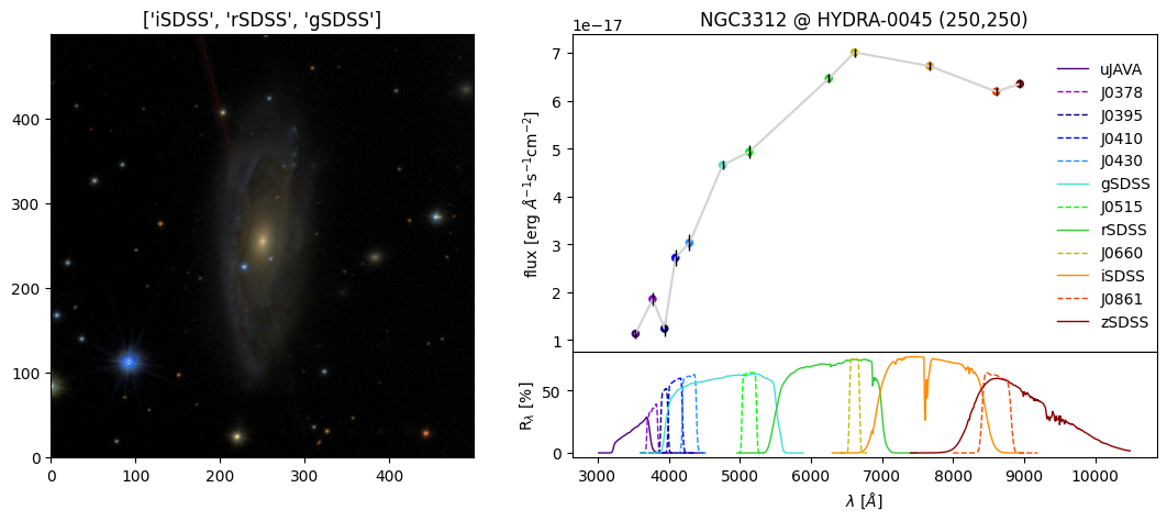
from matplotlib.gridspec import GridSpec

from scubes.constants import FILTER_NAMES_FITS, FILTER_COLORS, FILTER_TRANSMITTANCE

# central coords
i_x0, i_y0 = scube.i_x0, scube.i_y0
spec_pix_y, spec_pix_x = i_y0, i_x0

# data
logflux__l = np.ma.log10(scube.flux__lyx[:, i_y0, i_x0])  #.sum(axis=(1, 2)))
logeflux__l = np.ma.log10(scube.eflux__lyx[:, i_y0, i_x0])
flux__l = scube.flux__lyx[:, i_y0, i_x0]
eflux__l = scube.eflux__lyx[:, i_y0, i_x0]
bands__l = scube.pivot_wave

# plot
nrows = 4
ncols = 2
f = plt.figure()
f.set_size_inches(12, 5)
f.subplots_adjust(left=0, right=0.9)
gs = GridSpec(nrows=nrows, ncols=ncols, hspace=0, wspace=0.03, figure=f)
ax = f.add_subplot(gs[0:nrows - 1, 1])
axf = f.add_subplot(gs[-1, 1])
axrgb = f.add_subplot(gs[:, 0])

# RGB image
rgb__yxb = scube.lRGB_image(
    rgb=['iSDSS', 'rSDSS', 'gSDSS'], rgb_f=[1, 1, 1],
    pminmax=[5, 95], Q=10, stretch=5, im_max=1, minimum=(0, 0, 0)
)
axrgb.imshow(rgb__yxb, origin='lower')
axrgb.set_title(rgb)

# filters transmittance
filter_colors = []
axf.sharex(ax)
for k in scube.filters:
    _f = FILTER_TRANSMITTANCE[k]
    c = FILTER_COLORS[FILTER_NAMES_FITS[k]]
    filter_colors.append(c)
    lt = '--'
    if 'JAVA' in k or 'SDSS' in k:
        lt = '-'
    axf.plot(_f['wavelength'], _f['transmittance'], c=c, lw=1, ls=lt, label=k)
axf.legend(loc=(0.82, 1.15), frameon=False)

# spectrum
ax.set_title(f'{scube.galaxy} @ {scube.tile} ({spec_pix_x},{spec_pix_y})')
ax.plot(bands__l, flux__l, ':', c='k')
ax.scatter(bands__l, flux__l, c=np.array(filter_colors), s=0.5)
ax.errorbar(x=bands__l,y=flux__l, yerr=eflux__l, c='k', lw=1, fmt='|')
ax.plot(bands__l, flux__l, '-', c='lightgray')
ax.scatter(bands__l, flux__l, c=np.array(filter_colors))

ax.set_xlabel(r'$\lambda_{\rm pivot}\ [\AA]$', fontsize=10)
ax.set_ylabel(r'flux $[{\rm erg}\ \AA^{-1}{\rm s}^{-1}{\rm cm}^{-2}]$', fontsize=10)
axf.set_xlabel(r'$\lambda\ [\AA]$', fontsize=10)
axf.set_ylabel(r'${\rm R}_\lambda\ [\%]$', fontsize=10)
Text(0, 0.5, '${\rm R}_\lambda\ [\%]$')
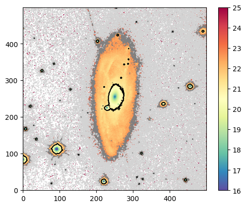
# Contour plot example
i_lambda = scube.filters.index('rSDSS')
image__yx = scube.mag__lyx[i_lambda]
contour_levels = [21, 23, 24]

f = plt.figure()
im = plt.imshow(image__yx, cmap='Spectral_r', origin='lower', vmin=16, vmax=25)
plt.contour(image__yx, levels=contour_levels, colors=['k', 'gray', 'lightgray'])
plt.colorbar(im)
<matplotlib.colorbar.Colorbar at 0x726e7e063df0>
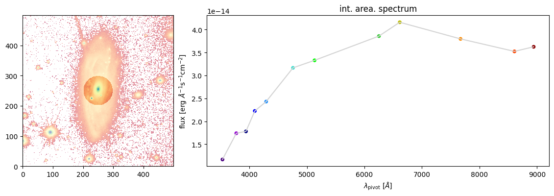
Distance from center
With scube.pixel_distance__yx property, the user also can play with
distance masks, such as create integrated spectra. An example:
from matplotlib.gridspec import GridSpec

max_dist = 50  # pixels
mask__yx = scube.pixel_distance__yx > max_dist
__lyx = (scube.n_filters, scube.n_y, scube.n_x)
mask__lyx = np.broadcast_to(mask__yx, __lyx)
integrated_flux__lyx = np.ma.masked_array(scube.flux__lyx, mask=mask__lyx, copy=True)

f = plt.figure()
f.set_size_inches(12, 4)
f.subplots_adjust(left=0, right=0.9)
gs = GridSpec(nrows=1, ncols=3, wspace=0.2, figure=f)
ax = f.add_subplot(gs[1:])
axmask = f.add_subplot(gs[0])
img__yx = np.ma.masked_array(scube.mag__lyx[scube.filters.index('rSDSS')], mask=mask__yx, copy=True)
im = axmask.imshow(img__yx, origin='lower', cmap='Spectral_r')
axmask.imshow(scube.mag__lyx[scube.filters.index('rSDSS')], origin='lower', cmap='Spectral_r', alpha=0.5, vmin=16, vmax=25)
bands__l = scube.pivot_wave
flux__l = integrated_flux__lyx.sum(axis=(1,2))
ax.plot(bands__l, flux__l, '-', c='lightgray')
ax.scatter(bands__l, flux__l, c=np.array(filter_colors), s=20, label='')
ax.set_xlabel(r'$\lambda_{\rm pivot}\ [\AA]$', fontsize=10)
ax.set_ylabel(r'flux $[{\rm erg}\ \AA^{-1}{\rm s}^{-1}{\rm cm}^{-2}]$', fontsize=10)
ax.set_title('int. area. spectrum')
Text(0.5, 1.0, 'int. area. spectrum')